Tip

An interactive online version of this notebook is available, which can be accessed via

---

Alternatively, you may download this notebook and run it offline.

Attention

You are viewing this notebook on the latest version of the documentation, where these notebooks may not be compatible with the stable release of PyBaMM since they can contain features that are not yet released. We recommend viewing these notebooks from the stable version of the documentation. To install the latest version of PyBaMM that is compatible with the latest notebooks, build PyBaMM from source.

Speeding up the solvers

This notebook contains a collection of tips on how to speed up the solvers

%pip install "pybamm[plot,cite]" -q    # install PyBaMM if it is not installed
import pybamm
import matplotlib.pyplot as plt
import numpy as np

Note: you may need to restart the kernel to use updated packages.

Choosing a solver

Since it is very easy to switch which solver is used for the model, we recommend you try different solvers for your particular use case. In general, the CasadiSolver is the fastest.

Once you have found a good solver, you can further improve performance by trying out different values for the method, rtol, and atol arguments. Further options are sometimes available, but are solver specific. See solver API docs for details.

Choosing and optimizing CasadiSolver settings

Fast mode vs safe mode

The CasadiSolver comes with a mode argument which can be set to “fast” or “safe” (the third option, “safe without grid”, is experimental and should not be used for now). The “fast” mode is faster but ignores any “events” (such as a voltage cut-off point), while the “safe” mode is slower but does stop at events (with manually implemented “step-and-check” under the hood). Therefore, “fast” mode should be used whenever events are not expected to be hit (for example, when simulating a drive cycle or a constant-current discharge where the time interval is such that the simulation will finish before reaching the voltage cut-off). Conversely, “safe” mode should be used whenever events are important: in particular, when using the Experiment class.

To demonstrate the difference between safe mode and fast mode, consider the following example

# Set up model
model = pybamm.lithium_ion.DFN()
param = model.default_parameter_values
cap = param["Nominal cell capacity [A.h]"]
param["Current function [A]"] = cap * pybamm.InputParameter("Crate")
sim = pybamm.Simulation(model, parameter_values=param)

# Set up solvers. Reduce max_num_steps for the fast solver, for faster errors
fast_solver = pybamm.CasadiSolver(
    mode="fast", extra_options_setup={"max_num_steps": 1000}
)
safe_solver = pybamm.CasadiSolver(mode="safe")

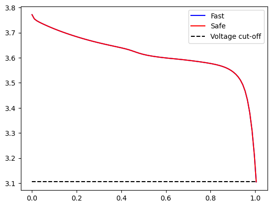
Both solvers can solve the model up to 3700 s, but the fast solver ignores the voltage cut-off around 3.1 V

safe_sol = sim.solve([0, 3700], solver=safe_solver, inputs={"Crate": 1})
fast_sol = sim.solve([0, 3700], solver=fast_solver, inputs={"Crate": 1})

timer = pybamm.Timer()
print("Safe:", safe_sol.solve_time)
print("Fast:", fast_sol.solve_time)

cutoff = param["Lower voltage cut-off [V]"]
plt.plot(fast_sol["Time [h]"].data, fast_sol["Voltage [V]"].data, "b-", label="Fast")
plt.plot(safe_sol["Time [h]"].data, safe_sol["Voltage [V]"].data, "r-", label="Safe")
plt.plot(
    fast_sol["Time [h]"].data,
    cutoff * np.ones_like(fast_sol["Time [h]"].data),
    "k--",
    label="Voltage cut-off",
)
plt.legend();

Safe: 161.060 ms
Fast: 78.290 ms

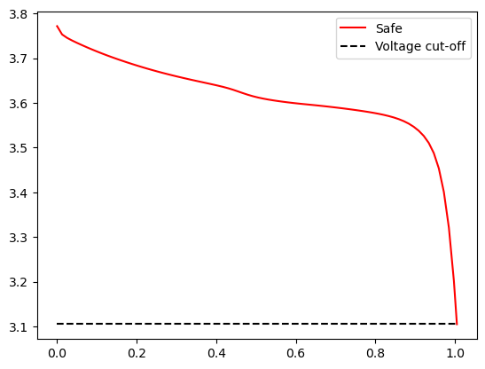
If we increase the integration interval, the safe solver still stops at the same point, but the fast solver fails

safe_sol = sim.solve([0, 4500], solver=safe_solver, inputs={"Crate": 1})

print("Safe:", safe_sol.solve_time)

plt.plot(safe_sol["Time [h]"].data, safe_sol["Voltage [V]"].data, "r-", label="Safe")
plt.plot(
    safe_sol["Time [h]"].data,
    cutoff * np.ones_like(safe_sol["Time [h]"].data),
    "k--",
    label="Voltage cut-off",
)
plt.legend()

try:
    sim.solve([0, 4500], solver=fast_solver, inputs={"Crate": 1})
except pybamm.SolverError as e:
    print("Solving fast mode, error occurred:", e.args[0])

At t = 506.167, , mxstep steps taken before reaching tout.

Safe: 7.181 s
Solving fast mode, error occurred: Error in Function::call for 'F' [IdasInterface] at .../casadi/core/function.cpp:1401:
Error in Function::call for 'F' [IdasInterface] at .../casadi/core/function.cpp:330:
.../casadi/interfaces/sundials/idas_interface.cpp:596: IDASolve returned "IDA_TOO_MUCH_WORK". Consult IDAS documentation.

At t = 4051.62, , mxstep steps taken before reaching tout.

We can solve with fast mode up to close to this time to understand why the model is failing

fast_sol = sim.solve([0, 4049], solver=fast_solver, inputs={"Crate": 1})
fast_sol.plot(
    [
        "Minimum negative particle surface concentration",
        "Electrolyte concentration [mol.m-3]",
        "Maximum positive particle surface concentration",
        "Voltage [V]",
    ],
    time_unit="seconds",
    figsize=(9, 9),
);

In this case, we can see that the reason the solver is failing is that the concentration at the surface of the particles in the positive electrode hit their maximum value of c_max. Since the exchange current density has a term sqrt(c_max-c_s_surf), the square root of a negative number is complex, c_s_surf going above c_max will cause the solver to fail.

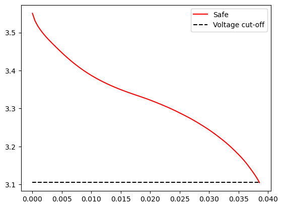
As a final note, there are some cases where the “safe” mode prints some warnings. This is linked to how the solver looks for events (sometimes stepping too far), and can be safely ignored if the solution looks sensible.

safe_sol_160 = sim.solve([0, 160], solver=safe_solver, inputs={"Crate": 10})
plt.plot(
    safe_sol_160["Time [h]"].data, safe_sol_160["Voltage [V]"].data, "r-", label="Safe"
)
plt.plot(
    safe_sol_160["Time [h]"].data,
    cutoff * np.ones_like(safe_sol_160["Time [h]"].data),
    "k--",
    label="Voltage cut-off",
)
plt.legend();

At t = 159.516 and h = 1.33464e-07, the corrector convergence failed repeatedly or with |h| = hmin.

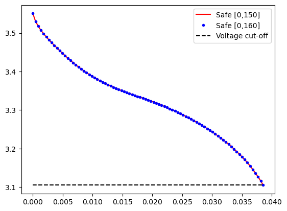
Reducing the time interval to [0, 150], we see that the solution is exactly the same, without the warnings

safe_sol_150 = sim.solve([0, 150], solver=safe_solver, inputs={"Crate": 10})
plt.plot(
    safe_sol_150["Time [h]"].data,
    safe_sol_150["Voltage [V]"].data,
    "r-",
    label="Safe [0,150]",
)
plt.plot(
    safe_sol_160["Time [h]"].data,
    safe_sol_160["Voltage [V]"].data,
    "b.",
    label="Safe [0,160]",
)
plt.plot(
    safe_sol_150["Time [h]"].data,
    cutoff * np.ones_like(safe_sol_150["Time [h]"].data),
    "k--",
    label="Voltage cut-off",
)
plt.legend();

safe_solver_2 = pybamm.CasadiSolver(mode="safe", dt_max=30)
safe_sol_2 = sim.solve([0, 160], solver=safe_solver_2, inputs={"Crate": 10})

Choosing dt_max to speed up the safe mode

The parameter dt_max controls how large the steps taken by the CasadiSolver with “safe” mode are when looking for events.

for dt_max in [10, 20, 100, 1000, 3700]:
    safe_sol = sim.solve(
        [0, 3600],
        solver=pybamm.CasadiSolver(mode="safe", dt_max=dt_max),
        inputs={"Crate": 1},
    )
    print(
        f"With dt_max={dt_max}, took {safe_sol.solve_time} "
        + f"(integration time: {safe_sol.integration_time})"
    )

fast_sol = sim.solve([0, 3600], solver=fast_solver, inputs={"Crate": 1})
print(
    f"With 'fast' mode, took {fast_sol.solve_time} "
    + f"(integration time: {fast_sol.integration_time})"
)

With dt_max=10, took 575.783 ms (integration time: 508.473 ms)
With dt_max=20, took 575.500 ms (integration time: 510.705 ms)
With dt_max=100, took 316.721 ms (integration time: 275.459 ms)
With dt_max=1000, took 76.646 ms (integration time: 49.294 ms)
With dt_max=3700, took 48.773 ms (integration time: 32.436 ms)
With 'fast' mode, took 42.224 ms (integration time: 32.177 ms)

In general, a larger value of dt_max gives a faster solution, since fewer integrator creations and calls are required.

Below the solution time interval of 36s, the value of dt_max does not affect the solve time, since steps must be at least 36s large. The discrepancy between the solve time and integration time is due to the extra operations recorded by “solve time”, such as creating the integrator. The “fast” solver does not need to do this (it reuses the first one it had already created), so the solve time is much closer to the integration time.

The example above was a case where no events are triggered, so the largest dt_max works well. If we step over events, then it is possible to makes dt_max too large, so that the solver will attempt (and fail) to take large steps past the event, iteratively reducing the step size until it works. For example:

for dt_max in [10, 20, 100, 1000, 3600]:
    # Reduce max_num_steps to fail faster
    safe_sol = sim.solve(
        [0, 4500],
        solver=pybamm.CasadiSolver(
            mode="safe", dt_max=dt_max, extra_options_setup={"max_num_steps": 1000}
        ),
        inputs={"Crate": 1},
    )
    print(
        f"With dt_max={dt_max}, took {safe_sol.solve_time} "
        + f"(integration time: {safe_sol.integration_time})"
    )

With dt_max=10, took 504.163 ms (integration time: 419.740 ms)
With dt_max=20, took 504.691 ms (integration time: 421.396 ms)
With dt_max=100, took 286.620 ms (integration time: 238.390 ms)
With dt_max=1000, took 98.500 ms (integration time: 60.880 ms)

At t = 460.712, , mxstep steps taken before reaching tout.
At t = 460.712 and h = 1.26752e-15, the corrector convergence failed repeatedly or with |h| = hmin.
At t = 460.712 and h = 9.51455e-16, the corrector convergence failed repeatedly or with |h| = hmin.

With dt_max=3600, took 645.118 ms (integration time: 32.601 ms)

The integration time with dt_max=3600 remains the fastest, but the solve time is the slowest due to all the failed steps.

Choosing the period for faster experiments

The “period” argument of the experiments also affects how long the simulations take, for a similar reason to dt_max. Therefore, this argument can be manually tuned to speed up how long an experiment takes to solve.

We start with one cycle of CCCV

experiment = pybamm.Experiment(
    [
        "Discharge at C/10 for 10 hours or until 3.3 V",
        "Rest for 1 hour",
        "Charge at 1 A until 4.1 V",
        "Hold at 4.1 V until 50 mA",
        "Rest for 1 hour",
    ]
)
solver = pybamm.CasadiSolver(mode="safe", extra_options_setup={"max_num_steps": 1000})
sim = pybamm.Simulation(model, experiment=experiment, solver=solver)
sol = sim.solve()
print("Took ", sol.solve_time)

Took  693.344 ms

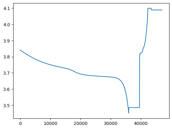
This gives a nice, smooth voltage curve

plt.plot(sol["Time [s]"].data, sol["Voltage [V]"].data);

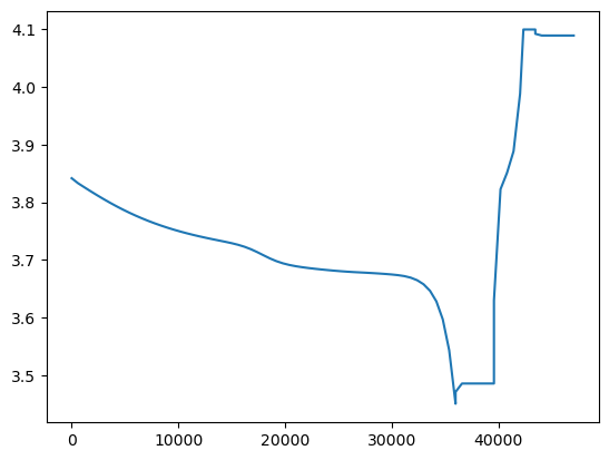
We can speed up the experiment by increasing the period, but tradeoff is that the resolution of the solution becomes worse

experiment = pybamm.Experiment(
    [
        "Discharge at C/10 for 10 hours or until 3.3 V",
        "Rest for 1 hour",
        "Charge at 1 A until 4.1 V",
        "Hold at 4.1 V until 50 mA",
        "Rest for 1 hour",
    ],
    period="10 minutes",
)
sim = pybamm.Simulation(model, experiment=experiment, solver=solver)
sol = sim.solve()
print("Took ", sol.solve_time)
plt.plot(sol["Time [s]"].data, sol["Voltage [V]"].data);

Took  598.237 ms

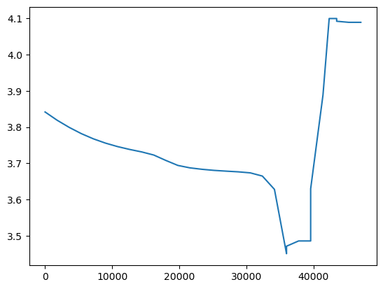
If we increase the period too much, the experiment becomes slower as the solver takes more failing steps

experiment = pybamm.Experiment(
    [
        "Discharge at C/10 for 10 hours or until 3.3 V",
        "Rest for 1 hour",
        "Charge at 1 A until 4.1 V",
        "Hold at 4.1 V until 50 mA",
        "Rest for 1 hour",
    ],
    period="30 minutes",
)
sim = pybamm.Simulation(model, experiment=experiment, solver=solver)
sol = sim.solve()
print("Took ", sol.solve_time)
plt.plot(sol["Time [s]"].data, sol["Voltage [V]"].data);

At t = 1262.29 and h = 3.51225e-14, the corrector convergence failed repeatedly or with |h| = hmin.

Took  532.042 ms

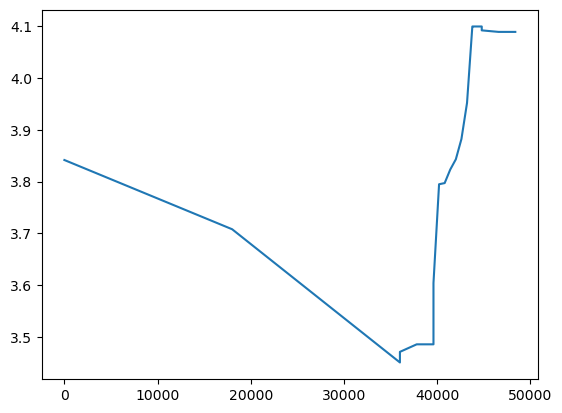
We can control the period of individual parts of the experiment to get the fastest solution (again, at the cost of resolution)

s = pybamm.step.string
experiment = pybamm.Experiment(
    [
        s("Discharge at C/10 for 10 hours or until 3.3 V", period="5 hours"),
        s("Rest for 1 hour", period="30 minutes"),
        s("Charge at 1 C until 4.1 V", period="10 minutes"),
        s("Hold at 4.1 V until 50 mA", period="10 minutes"),
        s("Rest for 1 hour", period="30 minutes"),
    ],
)
solver = pybamm.CasadiSolver(mode="safe", extra_options_setup={"max_num_steps": 1000})
sim = pybamm.Simulation(model, experiment=experiment, solver=solver)
sol = sim.solve()
print("Took ", sol.solve_time)
plt.plot(sol["Time [s]"].data, sol["Voltage [V]"].data);

Took  257.314 ms

As you can see, this kind of optimization requires a lot of manual tuning. We are working on ways to make the experiment class more efficient in general.

Changing the time interval

Finally, in some cases, changing the time interval (either the step size or the final time) may affect whether or not the casadi solver can solve the system. Therefore, if the casadi solver is failing, it may be worth changing the time interval (usually, reducing step size or final time) to see if that allows the solver to solve the model. Unfortunately, we have not yet been able to isolate a minimum working example to demonstrate this effect.

Handling instabilities

If the solver is taking a lot of steps, possibly failing with a max_steps error, and the error persists with different solvers and options, this suggests a problem with the model itself. This can be due to a few things:

• A singularity in the model (such as division by zero). Solve up to the time where the model fails, and plot some variables to see if they are going to infinity. You can then narrow down the source of the problem.

• High model stiffness. Set the scale parameter of variables so that their scaled nominal value (e.g. initial condition) is of order 1, and multiply algebraic equations by appropriate constants so that they are roughly of order 1.

• Non-differentiable functions (see below)

If none of these fixes work, we are interested in finding out why - please get in touch!

Smooth approximations to non-differentiable functions

Some functions, such as minimum, maximum, heaviside, and abs, are discontinuous and/or non-differentiable (their derivative is discontinuous). Adaptive solvers can deal with this discontinuity, but will take many more steps close to the discontinuity in order to resolve it. Therefore, using soft approximations instead can reduce the number of steps taken by the solver, and hence the integration time. See this post for more details.

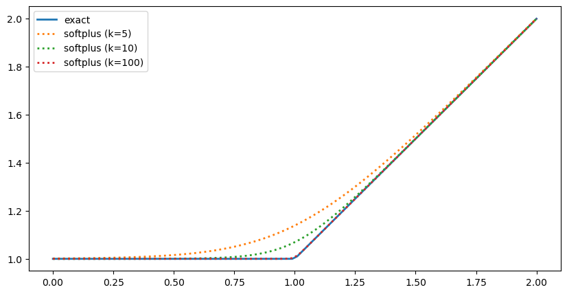
Here is an example using the maximum function. The function maximum(x,1) is continuous but non-differentiable at x=1, where its derivative jumps from 0 to 1. However, we can approximate it using the `softplus function <https://en.wikipedia.org/wiki/Rectifier_(neural_networks)#Softplus>`__, which is smooth everywhere and is sometimes used in neural networks as a smooth approximation to the RELU activation function. The softplus function is given by

\[s(x,y;k) = \frac{\log(\exp(kx)+\exp(ky))}{k},\]

where k is a strictly positive smoothing (or sharpness) parameter. The larger the value of k, the better the approximation but the stiffer the term (exp blows up quickly!). Usually, a value of k=10 is a good middle ground.

In PyBaMM, you can either call the softplus function directly, or change pybamm.settings.max_smoothing to automatically replace all your calls to pybamm.maximum with softplus.

x = pybamm.Variable("x")
y = pybamm.Variable("y")

# Normal maximum
print(f"Exact maximum: {pybamm.maximum(x,y)}")

# Softplus
print("Softplus (k=10): ", pybamm.softplus(x, y, 10))

# Changing the setting to call softplus automatically
pybamm.settings.min_max_mode = "soft"
pybamm.settings.min_max_smoothing = 20
print(f"Softplus (k=20): {pybamm.maximum(x,y)}")

# All smoothing parameters can be changed at once
pybamm.settings.set_smoothing_parameters(30)
print(f"Softplus (k=30): {pybamm.maximum(x,y)}")

# Change back
pybamm.settings.set_smoothing_parameters("exact")
print(f"Exact maximum: {pybamm.maximum(x,y)}")

Exact maximum: maximum(x, y)
Softplus (k=10):  0.1 * log(exp(10.0 * x) + exp(10.0 * y))
Softplus (k=20): 0.05 * log(exp(20.0 * x) + exp(20.0 * y))
Softplus (k=30): 0.03333333333333333 * log(exp(30.0 * x) + exp(30.0 * y))
Exact maximum: maximum(x, y)

Note that if both sides are constant then pybamm will use the exact value even if the setting is set to smoothing

a = pybamm.InputParameter("a")
pybamm.settings.max_smoothing = 20
# Both inputs are constant so uses exact maximum
print("Exact:", pybamm.maximum(0.999, 1).evaluate())
# One input is not constant (InputParameter) so uses softplus
print("Softplus:", pybamm.maximum(a, 1).evaluate(inputs={"a": 0.999}))
pybamm.settings.set_smoothing_parameters("exact")

Exact: 1.0
Softplus: 1.0

Here is the plot of softplus with different values of k

pts = pybamm.linspace(0, 2, 100)

fig, ax = plt.subplots(figsize=(10, 5))
ax.plot(pts.evaluate(), pybamm.maximum(pts, 1).evaluate(), lw=2, label="exact")
ax.plot(
    pts.evaluate(),
    pybamm.softplus(pts, 1, 5).evaluate(),
    ":",
    lw=2,
    label="softplus (k=5)",
)
ax.plot(
    pts.evaluate(),
    pybamm.softplus(pts, 1, 10).evaluate(),
    ":",
    lw=2,
    label="softplus (k=10)",
)
ax.plot(
    pts.evaluate(),
    pybamm.softplus(pts, 1, 100).evaluate(),
    ":",
    lw=2,
    label="softplus (k=100)",
)
ax.legend();

Solving a model with the exact maximum and soft approximation, demonstrates a clear speed-up even for a very simple model

model_exact = pybamm.BaseModel()
model_exact.rhs = {x: pybamm.maximum(x, 1)}
model_exact.initial_conditions = {x: 0.5}
model_exact.variables = {"x": x, "max(x,1)": pybamm.maximum(x, 1)}

model_smooth = pybamm.BaseModel()
k = pybamm.InputParameter("k")
model_smooth.rhs = {x: pybamm.softplus(x, 1, k)}
model_smooth.initial_conditions = {x: 0.5}
model_smooth.variables = {"x": x, "max(x,1)": pybamm.softplus(x, 1, k)}


# Exact solution
timer = pybamm.Timer()
time = 0
solver = pybamm.CasadiSolver(mode="fast")
for _ in range(100):
    exact_sol = solver.solve(model_exact, [0, 2])
    # Report integration time, which is the time spent actually doing the integration
    time += exact_sol.integration_time
print("Exact:", time / 100)
sols = [exact_sol]

ks = [5, 10, 100]
solver = pybamm.CasadiSolver(mode="fast")
for k in ks:
    time = 0
    for _ in range(100):
        sol = solver.solve(model_smooth, [0, 2], inputs={"k": k})
        time += sol.integration_time
    print(f"Soft, k={k}:", time / 100)
    sols.append(sol)

pybamm.dynamic_plot(
    sols, ["x", "max(x,1)"], labels=["exact"] + [f"soft (k={k})" for k in ks]
);

Exact: 172.706 us
Soft, k=5: 160.098 us
Soft, k=10: 133.737 us
Soft, k=100: 168.833 us

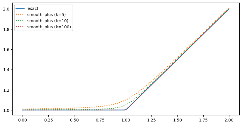
For the minimum and maximum functions, an alternative smoothing functions (smooth_max, smooth_min) are provided.

\[\textrm{min}(x, y) = 0.5 * (\sqrt((x - y)^2 + \sigma) + (x + y)) \quad , \quad \textrm{max}(x, y) = 0.5 * ((x + y) - \sqrt((x - y)^2 + \sigma))\]

where

\[\sigma = \frac{1}{k^2}\]

For the smooth minimum and maximum functions, the recommended value of k is 100, where the function closely approximates the exact function, but is differentiable.

Changing between the soft, smooth, and exact functions can be done by setting the min_max_mode and the value of k stored in min_max_smoothing

x = pybamm.Variable("x")
y = pybamm.Variable("y")

# Normal maximum
print(f"Exact maximum: {pybamm.maximum(x,y)}")

# Smooth plus can be called explicitly
print("Smooth plus (k=100): ", pybamm.smooth_max(x, y, 100))

# Smooth plus and smooth minus will be used when the mode is set to "smooth"
pybamm.settings.min_max_mode = "smooth"
pybamm.settings.min_max_smoothing = 200
print(f"Smooth plus (k=200): {pybamm.maximum(x,y)}")

# Setting the smoothing parameters with set_smoothing_parameters() defaults to softplus
pybamm.settings.set_smoothing_parameters(10)
print(f"Softplus (k=10): {pybamm.maximum(x,y)}")

# Change back
pybamm.settings.set_smoothing_parameters("exact")
print(f"Exact maximum: {pybamm.maximum(x,y)}")

Exact maximum: maximum(x, y)
Smooth plus (k=100):  0.5 * (sqrt(0.0001 + (x - y) ** 2.0) + x + y)
Smooth plus (k=200): 0.5 * (sqrt(2.5e-05 + (x - y) ** 2.0) + x + y)
Softplus (k=10): 0.1 * log(exp(10.0 * x) + exp(10.0 * y))
Exact maximum: maximum(x, y)

Here is the plot of smooth_max with different values of k

pts = pybamm.linspace(0, 2, 100)

fig, ax = plt.subplots(figsize=(10, 5))
ax.plot(pts.evaluate(), pybamm.maximum(pts, 1).evaluate(), lw=2, label="exact")
ax.plot(
    pts.evaluate(),
    pybamm.smooth_max(pts, 1, 5).evaluate(),
    ":",
    lw=2,
    label="smooth_max (k=5)",
)
ax.plot(
    pts.evaluate(),
    pybamm.smooth_max(pts, 1, 10).evaluate(),
    ":",
    lw=2,
    label="smooth_max (k=10)",
)
ax.plot(
    pts.evaluate(),
    pybamm.smooth_max(pts, 1, 100).evaluate(),
    ":",
    lw=2,
    label="smooth_max (k=100)",
)
ax.legend();

Solving a model with the exact maximum and smooth approximation, demonstrates a clear speed-up even for a very simple model

model_exact = pybamm.BaseModel()
model_exact.rhs = {x: pybamm.maximum(x, 1)}
model_exact.initial_conditions = {x: 0.5}
model_exact.variables = {"x": x, "max(x,1)": pybamm.maximum(x, 1)}

model_smooth = pybamm.BaseModel()
k = pybamm.InputParameter("k")
model_smooth.rhs = {x: pybamm.smooth_max(x, 1, k)}
model_smooth.initial_conditions = {x: 0.5}
model_smooth.variables = {"x": x, "max(x,1)": pybamm.smooth_max(x, 1, k)}


# Exact solution
timer = pybamm.Timer()
time = 0
solver = pybamm.CasadiSolver(mode="fast")
for _ in range(100):
    exact_sol = solver.solve(model_exact, [0, 2])
    # Report integration time, which is the time spent actually doing the integration
    time += exact_sol.integration_time
print("Exact:", time / 100)
sols = [exact_sol]

ks = [10, 50, 100, 1000, 10000]
solver = pybamm.CasadiSolver(mode="fast")
for k in ks:
    time = 0
    for _ in range(100):
        sol = solver.solve(model_smooth, [0, 2], inputs={"k": k})
        time += sol.integration_time
    print(f"Smooth, k={k}:", time / 100)
    sols.append(sol)

pybamm.dynamic_plot(
    sols, ["x", "max(x,1)"], labels=["exact"] + [f"soft (k={k})" for k in ks]
);

Exact: 168.348 us
Smooth, k=10: 149.515 us
Smooth, k=50: 170.092 us
Smooth, k=100: 137.928 us
Smooth, k=1000: 200.991 us
Smooth, k=10000: 175.300 us

Other smooth approximations

Here are the other smooth approximations for the other non-smooth functions:

pybamm.settings.set_smoothing_parameters(10)
print(f"Soft minimum (softminus):\t {pybamm.minimum(x,y)!s}")
print(f"Smooth heaviside (sigmoid):\t {x < y!s}")
print(f"Smooth absolute value: \t\t {abs(x)!s}")
pybamm.settings.min_max_mode = "smooth"
print(f"Smooth minimum:\t\t\t {pybamm.minimum(x,y)!s}")
pybamm.settings.set_smoothing_parameters("exact")

Soft minimum (softminus):        -0.1 * log(exp(-10.0 * x) + exp(-10.0 * y))
Smooth heaviside (sigmoid):      0.5 + 0.5 * tanh(10.0 * (y - x))
Smooth absolute value:           x * (exp(10.0 * x) - exp(-10.0 * x)) / (exp(10.0 * x) + exp(-10.0 * x))
Smooth minimum:                  0.5 * (x + y - sqrt(0.010000000000000002 + (x - y) ** 2.0))

References

The relevant papers for this notebook are:

pybamm.print_citations()

[1] Joel A. E. Andersson, Joris Gillis, Greg Horn, James B. Rawlings, and Moritz Diehl. CasADi – A software framework for nonlinear optimization and optimal control. Mathematical Programming Computation, 11(1):1–36, 2019. doi:10.1007/s12532-018-0139-4.
[2] Marc Doyle, Thomas F. Fuller, and John Newman. Modeling of galvanostatic charge and discharge of the lithium/polymer/insertion cell. Journal of the Electrochemical society, 140(6):1526–1533, 1993. doi:10.1149/1.2221597.
[3] Charles R. Harris, K. Jarrod Millman, Stéfan J. van der Walt, Ralf Gommers, Pauli Virtanen, David Cournapeau, Eric Wieser, Julian Taylor, Sebastian Berg, Nathaniel J. Smith, and others. Array programming with NumPy. Nature, 585(7825):357–362, 2020. doi:10.1038/s41586-020-2649-2.
[4] Scott G. Marquis, Valentin Sulzer, Robert Timms, Colin P. Please, and S. Jon Chapman. An asymptotic derivation of a single particle model with electrolyte. Journal of The Electrochemical Society, 166(15):A3693–A3706, 2019. doi:10.1149/2.0341915jes.
[5] Peyman Mohtat, Suhak Lee, Jason B Siegel, and Anna G Stefanopoulou. Towards better estimability of electrode-specific state of health: decoding the cell expansion. Journal of Power Sources, 427:101–111, 2019.
[6] Valentin Sulzer, Scott G. Marquis, Robert Timms, Martin Robinson, and S. Jon Chapman. Python Battery Mathematical Modelling (PyBaMM). Journal of Open Research Software, 9(1):14, 2021. doi:10.5334/jors.309.
[7] Pauli Virtanen, Ralf Gommers, Travis E. Oliphant, Matt Haberland, Tyler Reddy, David Cournapeau, Evgeni Burovski, Pearu Peterson, Warren Weckesser, Jonathan Bright, and others. SciPy 1.0: fundamental algorithms for scientific computing in Python. Nature Methods, 17(3):261–272, 2020. doi:10.1038/s41592-019-0686-2.
[8] Andrew Weng, Jason B Siegel, and Anna Stefanopoulou. Differential voltage analysis for battery manufacturing process control. arXiv preprint arXiv:2303.07088, 2023.