Tip

An interactive online version of this notebook is available, which can be accessed via

---

Alternatively, you may download this notebook and run it offline.

Attention

You are viewing this notebook on the latest version of the documentation, where these notebooks may not be compatible with the stable release of PyBaMM since they can contain features that are not yet released. We recommend viewing these notebooks from the stable version of the documentation. To install the latest version of PyBaMM that is compatible with the latest notebooks, build PyBaMM from source.

%pip install "pybamm[plot,cite]" -q    # install PyBaMM if it is not installed
import pybamm
import numpy as np

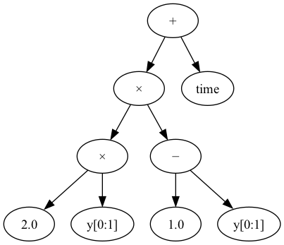
y = pybamm.StateVector(slice(0, 1))
t = pybamm.t
equation = 2 * y * (1 - y) + t
equation.visualise("expression_tree1.png")

Note: you may need to restart the kernel to use updated packages.

Once the equation is constructed, we can evaluate it at a given \(t=1\) and \(\mathbf{y}=\begin{pmatrix} 2 \end{pmatrix}\).

equation.evaluate(1, np.array([2]))

array([[-3.]])

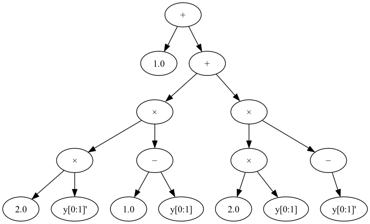
We can also calculate the expression tree representing the gradient of the equation with respect to \(t\),

diff_wrt_equation = equation.diff(t)
diff_wrt_equation.visualise("expression_tree2.png")

…and evaluate this expression,

diff_wrt_equation.evaluate(t=1, y=np.array([2]), y_dot=np.array([2]))

array([[-11.]])

The PyBaMM Pipeline

Proposing, parameter setting and discretising a model in PyBaMM is a pipeline process, consisting of the following steps:

1. The model is proposed, consisting of equations representing the right-hand-side of an ordinary differential equation (ODE), and/or algebraic equations for a differential algebraic equation (DAE), and also associated boundary condition equations

2. The parameters present in the model are replaced by actual scalar values from a parameter file, using the `pybamm.ParameterValues <https://docs.pybamm.org/en/latest/source/api/parameters/parameter_values.html>`__ class

3. The equations in the model are discretised onto a mesh, any spatial gradients are replaced with linear algebra expressions and the variables of the model are replaced with state vector slices. This is done using the `pybamm.Discretisation <https://docs.pybamm.org/en/latest/source/api/spatial_methods/discretisation.html>`__ class.

Stage 1 - Symbolic Expression Trees

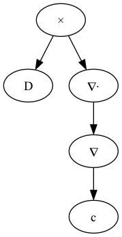
At each stage, the expression tree consists of certain types of nodes. In the first stage, the model is first proposed using `pybamm.Parameter <https://docs.pybamm.org/en/latest/source/api/expression_tree/parameter.html>`__, `pybamm.Variable <https://docs.pybamm.org/en/latest/source/api/expression_tree/variable.html>`__, and other unary and binary operators (which also includes spatial operators such as `pybamm.Gradient <https://docs.pybamm.org/en/latest/source/api/expression_tree/unary_operator.html#pybamm.Gradient>`__ and `pybamm.Divergence <https://docs.pybamm.org/en/latest/source/api/expression_tree/unary_operator.html#pybamm.Divergence>`__). For example, the right hand side of the equation

\[\frac{d c}{dt} = D \nabla \cdot \nabla c\]

can be constructed as an expression tree like so:

D = pybamm.Parameter("D")
c = pybamm.Variable("c", domain=["negative electrode"])

dcdt = D * pybamm.div(pybamm.grad(c))
dcdt.visualise("expression_tree3.png")

Stage 2 - Setting parameters

In the second stage, the pybamm.ParameterValues class is used to replace all the parameter nodes with scalar values, according to an input parameter file. For example, we’ll use a this class to set \(D = 2\)

parameter_values = pybamm.ParameterValues({"D": 2})
dcdt = parameter_values.process_symbol(dcdt)
dcdt.visualise("expression_tree4.png")

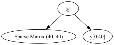
Stage 3 - Linear Algebra Expression Trees

The third and final stage uses the pybamm.Discretisation class to discretise the spatial gradients and variables over a given mesh. After this stage the expression tree will encode a linear algebra expression that can be evaluated given the state vector \(\mathbf{y}\) and \(t\).

Note: for demonstration purposes, we use a dummy discretisation below. For a more complete description of the pybamm.Discretisation class, see the example notebook here.

# Here, we import a dummy discretisation from the PyBaMM tests directory.
import sys

sys.path.insert(0, pybamm.root_dir())
from tests import get_discretisation_for_testing

disc = get_discretisation_for_testing()
disc.y_slices = {c: [slice(0, 40)]}
dcdt = disc.process_symbol(dcdt)
dcdt.visualise("expression_tree5.png")

After the third stage, our expression tree is now able to be evaluated by one of the solver classes. Note that we have used a single equation above to illustrate the different types of expression trees in PyBaMM, but any given models will consist of many RHS or algebraic equations, along with boundary conditions. See here for more details of PyBaMM models.

References

The relevant papers for this notebook are:

pybamm.print_citations()

[1] Charles R. Harris, K. Jarrod Millman, Stéfan J. van der Walt, Ralf Gommers, Pauli Virtanen, David Cournapeau, Eric Wieser, Julian Taylor, Sebastian Berg, Nathaniel J. Smith, and others. Array programming with NumPy. Nature, 585(7825):357–362, 2020. doi:10.1038/s41586-020-2649-2.
[2] Valentin Sulzer, Scott G. Marquis, Robert Timms, Martin Robinson, and S. Jon Chapman. Python Battery Mathematical Modelling (PyBaMM). Journal of Open Research Software, 9(1):14, 2021. doi:10.5334/jors.309.