Tip

An interactive online version of this notebook is available, which can be accessed via

Alternatively, you may download this notebook and run it offline.

Attention

You are viewing this notebook on the latest version of the documentation, where these notebooks may not be compatible with the stable release of PyBaMM since they can contain features that are not yet released. We recommend viewing these notebooks from the stable version of the documentation. To install the latest version of PyBaMM that is compatible with the latest notebooks, build PyBaMM from source.

Comparing with Experimental Data#

In this notebook we show how to compare results generated in PyBaMM with experimental data. We compare the results of the DFN model (see the DFN notebook) with the experimental data from Ecker et. al. [3]. Results are compared for a constant current discharge at 1C and at 5C.

First we import pybamm and any other packages required by this example, and then change our working directory to the root of the pybamm folder.

[1]:

%pip install "pybamm[plot,cite]" -q    # install PyBaMM if it is not installed
import pybamm
import os
import pandas as pd
import numpy as np
import matplotlib.pyplot as plt

os.chdir(pybamm.__path__[0] + "/..")

Note: you may need to restart the kernel to use updated packages.

We then load the Ecker data in from the .csv files using pandas

[2]:

voltage_data_1C = pd.read_csv(
    "pybamm/input/discharge_data/Ecker2015/Ecker_1C.csv", header=None
).to_numpy()
voltage_data_5C = pd.read_csv(
    "pybamm/input/discharge_data/Ecker2015/Ecker_5C.csv", header=None
).to_numpy()

Note that the data is Time [s] vs Voltage [V].

We load the DFN model and select the parameter set from the Ecker paper [1]. We update the C-rate an InputParameter so that we can re-run the same model at different C-rates without the need to rebuild the model. This is done by passing the flag [input].

[3]:

# choose DFN
model = pybamm.lithium_ion.DFN()

# pick parameters, keeping C-rate as an input to be changed for each solve
parameter_values = pybamm.ParameterValues("Ecker2015")
parameter_values.update({"Current function [A]": "[input]"})

For this comparison we choose a fine mesh of 1 finite volume per micron in the electrodes and separator and 1 finite volume per 0.1 micron in the particles

[4]:

var = pybamm.standard_spatial_vars
var_pts = {
    var.x_n: int(parameter_values.evaluate(model.param.n.L / 1e-6)),
    var.x_s: int(parameter_values.evaluate(model.param.s.L / 1e-6)),
    var.x_p: int(parameter_values.evaluate(model.param.p.L / 1e-6)),
    var.r_n: int(parameter_values.evaluate(model.param.n.prim.R_typ / 1e-7)),
    var.r_p: int(parameter_values.evaluate(model.param.p.prim.R_typ / 1e-7)),
}

We create a simulation using our model, parameters and number of grid points

[5]:

sim = pybamm.Simulation(model, parameter_values=parameter_values, var_pts=var_pts)

We can then solve the model for a 1C and 5C discharge

[6]:

C_rates = [1, 5]  # C-rates to solve for
capacity = parameter_values["Nominal cell capacity [A.h]"]
t_evals = [
    np.linspace(0, 3800, 100),
    np.linspace(0, 720, 100),
]  # times to return the solution at
solutions = [None] * len(C_rates)  # empty list that will hold solutions

# loop over C-rates
for i, C_rate in enumerate(C_rates):
    current = C_rate * capacity
    sim.solve(
        t_eval=t_evals[i],
        solver=pybamm.CasadiSolver(mode="fast"),
        inputs={"Current function [A]": current},
    )
    solutions[i] = sim.solution

Finally we plot the numerical solution against the experimental data

[7]:

fig, (ax1, ax2) = plt.subplots(1, 2, figsize=(13, 4))

# plot the 1C results
t_sol = solutions[0]["Time [s]"].entries
ax1.plot(t_sol, solutions[0]["Voltage [V]"](t_sol))
ax1.plot(voltage_data_1C[:, 0], voltage_data_1C[:, 1], "o")
ax1.set_xlabel("Time [s]")
ax1.set_ylabel("Voltage [V]")
ax1.set_title("1C")
ax1.legend(["DFN", "Experiment"], loc="best")

# plot the 5C results
t_sol = solutions[1]["Time [s]"].entries
ax2.plot(t_sol, solutions[1]["Voltage [V]"](t_sol))
ax2.plot(voltage_data_5C[:, 0], voltage_data_5C[:, 1], "o")
ax2.set_xlabel("Time [s]")
ax2.set_ylabel("Voltage [V]")
ax2.set_title("5C")
ax2.legend(["DFN", "Experiment"], loc="best")

plt.tight_layout()
plt.show()

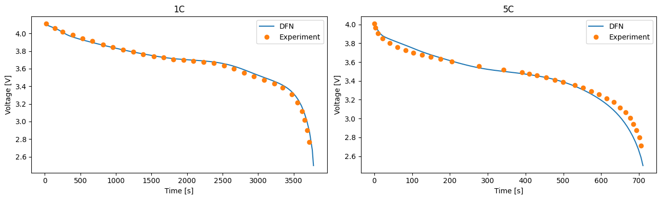
../../../../_images/source_examples_notebooks_models_compare-ecker-data_15_0.png

For a 1C discharge we observe an excellent agreement between the model and experiment, both in terms of the overall shape of the curve and the capacity. The agreement between model and experiment is less good at 5C, but in line with other implementations of the DFN (e.g. [6]).

References#

The relevant papers for this notebook are:

[8]:

pybamm.print_citations()

[1] Weilong Ai, Ludwig Kraft, Johannes Sturm, Andreas Jossen, and Billy Wu. Electrochemical thermal-mechanical modelling of stress inhomogeneity in lithium-ion pouch cells. Journal of The Electrochemical Society, 167(1):013512, 2019. doi:10.1149/2.0122001JES.
[2] Joel A. E. Andersson, Joris Gillis, Greg Horn, James B. Rawlings, and Moritz Diehl. CasADi – A software framework for nonlinear optimization and optimal control. Mathematical Programming Computation, 11(1):1–36, 2019. doi:10.1007/s12532-018-0139-4.
[3] Rutooj Deshpande, Mark Verbrugge, Yang-Tse Cheng, John Wang, and Ping Liu. Battery cycle life prediction with coupled chemical degradation and fatigue mechanics. Journal of the Electrochemical Society, 159(10):A1730, 2012. doi:10.1149/2.049210jes.
[4] Marc Doyle, Thomas F. Fuller, and John Newman. Modeling of galvanostatic charge and discharge of the lithium/polymer/insertion cell. Journal of the Electrochemical society, 140(6):1526–1533, 1993. doi:10.1149/1.2221597.
[5] Madeleine Ecker, Stefan Käbitz, Izaro Laresgoiti, and Dirk Uwe Sauer. Parameterization of a Physico-Chemical Model of a Lithium-Ion Battery: II. Model Validation. Journal of The Electrochemical Society, 162(9):A1849–A1857, 2015. doi:10.1149/2.0541509jes.
[6] Madeleine Ecker, Thi Kim Dung Tran, Philipp Dechent, Stefan Käbitz, Alexander Warnecke, and Dirk Uwe Sauer. Parameterization of a Physico-Chemical Model of a Lithium-Ion Battery: I. Determination of Parameters. Journal of the Electrochemical Society, 162(9):A1836–A1848, 2015. doi:10.1149/2.0551509jes.
[7] Alastair Hales, Laura Bravo Diaz, Mohamed Waseem Marzook, Yan Zhao, Yatish Patel, and Gregory Offer. The cell cooling coefficient: a standard to define heat rejection from lithium-ion batteries. Journal of The Electrochemical Society, 166(12):A2383, 2019.
[8] Charles R. Harris, K. Jarrod Millman, Stéfan J. van der Walt, Ralf Gommers, Pauli Virtanen, David Cournapeau, Eric Wieser, Julian Taylor, Sebastian Berg, Nathaniel J. Smith, and others. Array programming with NumPy. Nature, 585(7825):357–362, 2020. doi:10.1038/s41586-020-2649-2.
[9] Giles Richardson, Ivan Korotkin, Rahifa Ranom, Michael Castle, and Jamie M. Foster. Generalised single particle models for high-rate operation of graded lithium-ion electrodes: systematic derivation and validation. Electrochimica Acta, 339:135862, 2020. doi:10.1016/j.electacta.2020.135862.
[10] Valentin Sulzer, Scott G. Marquis, Robert Timms, Martin Robinson, and S. Jon Chapman. Python Battery Mathematical Modelling (PyBaMM). Journal of Open Research Software, 9(1):14, 2021. doi:10.5334/jors.309.
[11] Yan Zhao, Yatish Patel, Teng Zhang, and Gregory J Offer. Modeling the effects of thermal gradients induced by tab and surface cooling on lithium ion cell performance. Journal of The Electrochemical Society, 165(13):A3169, 2018.