Tip

An interactive online version of this notebook is available, which can be accessed via

---

Alternatively, you may download this notebook and run it offline.

Attention

You are viewing this notebook on the latest version of the documentation, where these notebooks may not be compatible with the stable release of PyBaMM since they can contain features that are not yet released. We recommend viewing these notebooks from the stable version of the documentation. To install the latest version of PyBaMM that is compatible with the latest notebooks, build PyBaMM from source.

Creating a simple PDE model

In the previous notebook we show how to create, discretise and solve an ODE model in pybamm. In this notebook we show how to create and solve a PDE problem, which will require meshing of the spatial domain.

As an example, we consider the problem of linear diffusion on a unit sphere,

\[\frac{\partial c}{\partial t} = \nabla \cdot (\nabla c),\]

with the following boundary and initial conditions:

\[\left.\frac{\partial c}{\partial r}\right\vert_{r=0} = 0, \quad \left.\frac{\partial c}{\partial r}\right\vert_{r=1} = 2, \quad \left.c\right\vert_{t=0} = 1.\]

As before, we begin by importing the PyBaMM library into this notebook, along with any other packages we require:

%pip install "pybamm[plot,cite]" -q    # install PyBaMM if it is not installed
import pybamm
import numpy as np
import matplotlib.pyplot as plt

Note: you may need to restart the kernel to use updated packages.

Setting up the model

As in the previous example, we start with a pybamm.BaseModel object and define our model variables. Since we are now solving a PDE we need to tell pybamm the domain each variable belongs to so that it can be discretised in space in the correct way. This is done by passing the keyword argument domain, and in this example we choose the domain “negative particle”.

model = pybamm.BaseModel()

c = pybamm.Variable("Concentration", domain="negative particle")

Note that we have given our variable the (useful) name “Concentration”, but the symbol representing this variable is simply c.

We then state out governing equations. Sometime it is useful to define intermediate quantities in order to express the governing equations more easily. In this example we define the flux, then define the rhs to be minus the divergence of the flux. The equation is then added to the dictionary model.rhs

N = -pybamm.grad(c)  # define the flux
dcdt = -pybamm.div(N)  # define the rhs equation

model.rhs = {c: dcdt}  # add the equation to rhs dictionary

Unlike ODE models, PDE models require both initial and boundary conditions. Similar to initial conditions, boundary conditions can be added using the dictionary model.boundary_conditions. Boundary conditions for each variable are provided as a dictionary of the form {side: (value, type), where, in 1D, side can be “left” or “right”, value is the value of the boundary conditions, and type is the type of boundary condition (at present, this can be “Dirichlet” or “Neumann”).

# initial conditions
model.initial_conditions = {c: pybamm.Scalar(1)}

# boundary conditions
lbc = pybamm.Scalar(0)
rbc = pybamm.Scalar(2)
model.boundary_conditions = {c: {"left": (lbc, "Neumann"), "right": (rbc, "Neumann")}}

Note that in our example the boundary conditions take constant values, but the value can be any valid pybamm expression.

Finally, we add any variables of interest to the dictionary model.variables

model.variables = {"Concentration": c, "Flux": N}

Using the model

Now the model is now completely defined all that remains is to discretise and solve. Since this model is a PDE we need to define the geometry on which it will be solved, and choose how to mesh the geometry and discretise in space.

Defining a geometry and mesh

We can define spatial variables in a similar way to how we defined model variables, providing a domain and a coordinate system. The geometry on which we wish to solve the model is defined using a nested dictionary. The first key is the domain name (here “negative particle”) and the entry is a dictionary giving the limits of the domain.

# define geometry
r = pybamm.SpatialVariable(
    "r", domain=["negative particle"], coord_sys="spherical polar"
)
geometry = {
    "negative particle": {r: {"min": pybamm.Scalar(0), "max": pybamm.Scalar(1)}}
}

We then create a uniform one-dimensional mesh with 20 points.

# mesh and discretise
submesh_types = {"negative particle": pybamm.Uniform1DSubMesh}
var_pts = {r: 20}
mesh = pybamm.Mesh(geometry, submesh_types, var_pts)

Example of meshes that do require parameters include the pybamm.Exponential1DSubMesh which clusters points close to one or both boundaries using an exponential rule. It takes a parameter which sets how closely the points are clustered together, and also lets the users select the side on which more points should be clustered. For example, to create a mesh with more nodes clustered to the right (i.e. the surface in the particle problem), using a stretch factor of 2, we pass an instance of the exponential submesh class and a dictionary of parameters into the MeshGenerator class as follows: pybamm.MeshGenerator(pybamm.Exponential1DSubMesh, submesh_params={"side": "right", "stretch": 2})

After defining a mesh we choose a spatial method. Here we choose the Finite Volume Method. We then set up a discretisation by passing the mesh and spatial methods to the class pybamm.Discretisation. The model is then processed, turning the variables into (slices of) a statevector, spatial variables into vector and spatial operators into matrix-vector multiplications.

spatial_methods = {"negative particle": pybamm.FiniteVolume()}
disc = pybamm.Discretisation(mesh, spatial_methods)
disc.process_model(model);

Now that the model has been discretised we are ready to solve.

Solving the model

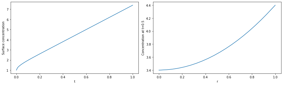
As before, we choose a solver and times at which we want the solution returned. We then solve, extract the variables we are interested in, and plot the result.

# solve
solver = pybamm.ScipySolver()
t = np.linspace(0, 1, 100)
solution = solver.solve(model, t)

# post-process, so that the solution can be called at any time t or space r
# (using interpolation)
c = solution["Concentration"]

# plot
fig, (ax1, ax2) = plt.subplots(1, 2, figsize=(13, 4))

ax1.plot(solution.t, c(solution.t, r=1))
ax1.set_xlabel("t")
ax1.set_ylabel("Surface concentration")
r = np.linspace(0, 1, 100)
ax2.plot(r, c(t=0.5, r=r))
ax2.set_xlabel("r")
ax2.set_ylabel("Concentration at t=0.5")
plt.tight_layout()
plt.show()

2021-11-19 15:31:50,774 - [WARNING] processed_variable.get_spatial_scale(520): No length scale set for negative particle. Using default of 1 [m].

In the next notebook we build on the example here to to solve the problem of diffusion in the negative electrode particle within the single particle model. In doing so we will also cover how to include parameters in a model.

References

The relevant papers for this notebook are:

pybamm.print_citations()

[1] Joel A. E. Andersson, Joris Gillis, Greg Horn, James B. Rawlings, and Moritz Diehl. CasADi – A software framework for nonlinear optimization and optimal control. Mathematical Programming Computation, 11(1):1–36, 2019. doi:10.1007/s12532-018-0139-4.
[2] Charles R. Harris, K. Jarrod Millman, Stéfan J. van der Walt, Ralf Gommers, Pauli Virtanen, David Cournapeau, Eric Wieser, Julian Taylor, Sebastian Berg, Nathaniel J. Smith, and others. Array programming with NumPy. Nature, 585(7825):357–362, 2020. doi:10.1038/s41586-020-2649-2.
[3] Valentin Sulzer, Scott G. Marquis, Robert Timms, Martin Robinson, and S. Jon Chapman. Python Battery Mathematical Modelling (PyBaMM). Journal of Open Research Software, 9(1):14, 2021. doi:10.5334/jors.309.
[4] Pauli Virtanen, Ralf Gommers, Travis E. Oliphant, Matt Haberland, Tyler Reddy, David Cournapeau, Evgeni Burovski, Pearu Peterson, Warren Weckesser, Jonathan Bright, and others. SciPy 1.0: fundamental algorithms for scientific computing in Python. Nature Methods, 17(3):261–272, 2020. doi:10.1038/s41592-019-0686-2.