Tip

An interactive online version of this notebook is available, which can be accessed via

Alternatively, you may download this notebook and run it offline.

Attention

You are viewing this notebook on the latest version of the documentation, where these notebooks may not be compatible with the stable release of PyBaMM since they can contain features that are not yet released. We recommend viewing these notebooks from the stable version of the documentation. To install the latest version of PyBaMM that is compatible with the latest notebooks, build PyBaMM from source.

Test the parameter set of the Enertech cells#

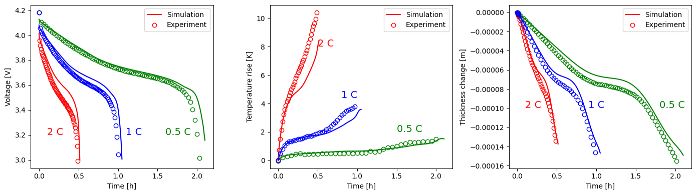
In this notebook, we show how to use pybamm to reproduce the experimental results for the Enertech cells (LCO-G). To see all of the models and submodels available in PyBaMM, please take a look at the documentation here.

[15]:

%pip install "pybamm[plot,cite]" -q    # install PyBaMM if it is not installed
import pybamm
import os
import matplotlib.pyplot as plt

os.chdir(pybamm.__path__[0] + "/..")

Note: you may need to restart the kernel to use updated packages.

Let’s load the DFN and include particle swelling

[16]:

model = pybamm.lithium_ion.DFN(
    options={
        "particle": "Fickian diffusion",
        "cell geometry": "arbitrary",
        "thermal": "lumped",
        "particle mechanics": "swelling only",
    }
)

We can get the parameter set Ai2020 for the model, which includes the mechanical properties required by the mechanical model.

[17]:

# update parameters, making C-rate and input
param = pybamm.ParameterValues("Ai2020")
capacity = param["Nominal cell capacity [A.h]"]
param.update({"Current function [A]": capacity * pybamm.InputParameter("C-rate")})

# update the mesh
var = pybamm.standard_spatial_vars
var_pts = {
    var.x_n: 50,
    var.x_s: 50,
    var.x_p: 50,
    var.r_n: 21,
    var.r_p: 21,
}

# define the simulation
sim = pybamm.Simulation(
    model,
    var_pts=var_pts,
    parameter_values=param,
    solver=pybamm.CasadiSolver(mode="fast"),
)

# solve for different C-rates
Crates = [0.5, 1, 2]
solutions = []
for Crate in Crates:
    print(f"{Crate} C")
    sol = sim.solve(t_eval=[0, 3600 / Crate * 1.05], inputs={"C-rate": Crate})
    solutions.append(sol)

# unpack solutions
solution05C, solution1C, solution2C = solutions

0.5 C
1 C
2 C

Load experimental results of the Enertech cells (see [1])

[18]:

# load experimental results
import pandas as pd

path = "pybamm/input/discharge_data/Enertech_cells/"
data_Disp_01C = pd.read_csv(
    path + "0.1C_discharge_displacement.txt", delimiter="\s+", header=None
)
data_Disp_05C = pd.read_csv(
    path + "0.5C_discharge_displacement.txt", delimiter="\s+", header=None
)
data_Disp_1C = pd.read_csv(
    path + "1C_discharge_displacement.txt", delimiter="\s+", header=None
)
data_Disp_2C = pd.read_csv(
    path + "2C_discharge_displacement.txt", delimiter="\s+", header=None
)
data_V_01C = pd.read_csv(path + "0.1C_discharge_U.txt", delimiter="\s+", header=None)
data_V_05C = pd.read_csv(path + "0.5C_discharge_U.txt", delimiter="\s+", header=None)
data_V_1C = pd.read_csv(path + "1C_discharge_U.txt", delimiter="\s+", header=None)
data_V_2C = pd.read_csv(path + "2C_discharge_U.txt", delimiter="\s+", header=None)
data_T_05C = pd.read_csv(path + "0.5C_discharge_T.txt", delimiter="\s+", header=None)
data_T_1C = pd.read_csv(path + "1C_discharge_T.txt", delimiter="\s+", header=None)
data_T_2C = pd.read_csv(path + "2C_discharge_T.txt", delimiter="\s+", header=None)

Plot the results.

[19]:

t_all2C = solution2C["Time [h]"].entries
V_n2C = solution2C["Voltage [V]"].entries
T_n2C = (
    solution2C["Volume-averaged cell temperature [K]"].entries
    - param["Initial temperature [K]"]
)
L_x2C = solution2C["Cell thickness change [m]"].entries

t_all1C = solution1C["Time [h]"].entries
V_n1C = solution1C["Voltage [V]"].entries
T_n1C = (
    solution1C["Volume-averaged cell temperature [K]"].entries
    - param["Initial temperature [K]"]
)
L_x1C = solution1C["Cell thickness change [m]"].entries

t_all05C = solution05C["Time [h]"].entries
V_n05C = solution05C["Voltage [V]"].entries
T_n05C = (
    solution05C["Volume-averaged cell temperature [K]"].entries
    - param["Initial temperature [K]"]
)
L_x05C = solution05C["Cell thickness change [m]"].entries

f, (ax1, ax2, ax3) = plt.subplots(1, 3, figsize=(14, 4))

ax1.plot(t_all2C, V_n2C, "r-", label="Simulation")
ax1.plot(
    data_V_2C.values[::30, 0] / 3600,
    data_V_2C.values[::30, 1],
    "ro",
    markerfacecolor="none",
    label="Experiment",
)
ax1.plot(t_all05C, V_n05C, "g-")
ax1.plot(
    data_V_05C.values[::100, 0] / 3600,
    data_V_05C.values[::100, 1],
    "go",
    markerfacecolor="none",
)
ax1.plot(t_all1C, V_n1C, "b-")
ax1.plot(
    data_V_1C.values[::50, 0] / 3600,
    data_V_1C.values[::50, 1],
    "bo",
    markerfacecolor="none",
)
ax1.legend()
ax1.set_xlabel("Time [h]")
ax1.set_ylabel("Voltage [V]")
ax1.text(0.1, 3.2, r"2 C", {"color": "r", "fontsize": 14})
ax1.text(1.1, 3.2, r"1 C", {"color": "b", "fontsize": 14})
ax1.text(1.6, 3.2, r"0.5 C", {"color": "g", "fontsize": 14})

ax2.plot(t_all2C, T_n2C, "r-", label="Simulation")
ax2.plot(
    data_T_2C.values[0:1754:50, 0] / 3600,
    data_T_2C.values[0:1754:50, 1],
    "ro",
    markerfacecolor="none",
    label="Experiment",
)
ax2.plot(t_all05C, T_n05C, "g-")
ax2.plot(
    data_T_05C.values[0:7301:200, 0] / 3600,
    data_T_05C.values[0:7301:200, 1],
    "go",
    markerfacecolor="none",
)
ax2.plot(t_all1C, T_n1C, "b-")
ax2.plot(
    data_T_1C.values[0:3598:100, 0] / 3600,
    data_T_1C.values[0:3598:100, 1],
    "bo",
    markerfacecolor="none",
)
ax2.legend()
ax2.set_xlabel("Time [h]")
ax2.set_ylabel("Temperature rise [K]")
ax2.text(0.5, 8, r"2 C", {"color": "r", "fontsize": 14})
ax2.text(0.8, 4.4, r"1 C", {"color": "b", "fontsize": 14})
ax2.text(1.5, 2, r"0.5 C", {"color": "g", "fontsize": 14})

ax3.plot(t_all2C, L_x2C, "r-", label="Simulation")
ax3.plot(
    data_Disp_2C.values[0:1754:5, 0] / 3600,
    data_Disp_2C.values[0:1754:5, 1] - data_Disp_2C.values[0, 1],
    "ro",
    markerfacecolor="none",
    label="Experiment",
)
ax3.plot(t_all05C, L_x05C, "g-")
ax3.plot(
    data_Disp_05C.values[0:1754:10, 0] / 3600,
    data_Disp_05C.values[0:1754:10, 1] - data_Disp_05C.values[0, 1],
    "go",
    markerfacecolor="none",
)
ax3.plot(t_all1C, L_x1C, "b-")
ax3.plot(
    data_Disp_1C.values[0:1754:10, 0] / 3600,
    data_Disp_1C.values[0:1754:10, 1] - data_Disp_1C.values[0, 1],
    "bo",
    markerfacecolor="none",
)
ax3.legend()
ax3.set_xlabel("Time [h]")
ax3.set_ylabel("Thickness change [m]")
ax3.text(0.1, -0.0001, r"2 C", {"color": "r", "fontsize": 14})
ax3.text(0.9, -0.0001, r"1 C", {"color": "b", "fontsize": 14})
ax3.text(1.8, -0.0001, r"0.5 C", {"color": "g", "fontsize": 14})

f.tight_layout()
f.show()

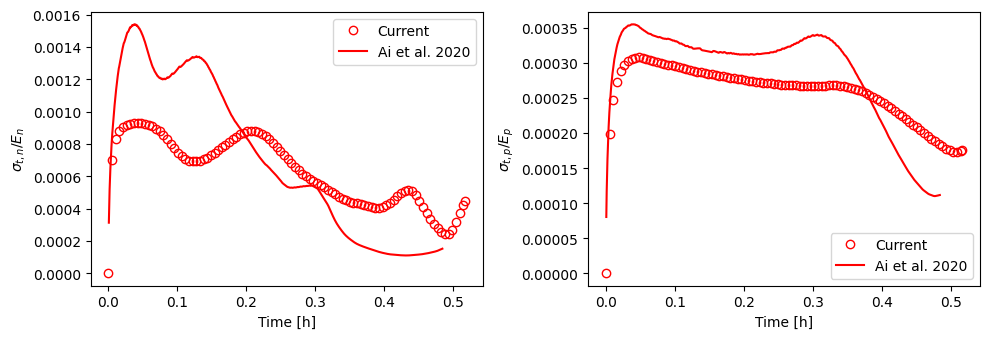
../../../../_images/source_examples_notebooks_models_Validating_mechanical_models_Enertech_DFN_9_0.png

Stress data below are from Fig. 6 in [1]

[20]:

E_n = param["Negative electrode Young's modulus [Pa]"]
E_p = param["Positive electrode Young's modulus [Pa]"]

cs_n_xav = solution2C["X-averaged negative particle concentration [mol.m-3]"].entries
cs_p_xav = solution2C["X-averaged positive particle concentration [mol.m-3]"].entries
st_surf_n = solution2C["Negative particle surface tangential stress [Pa]"].entries / E_n
st_surf_p = solution2C["Positive particle surface tangential stress [Pa]"].entries / E_p

data_st_n_2C = pd.read_csv(path + "stn_2C.txt", delimiter=",", header=3)
data_st_p_2C = pd.read_csv(path + "stp_2C.txt", delimiter=",", header=3)

f, (ax1, ax2) = plt.subplots(1, 2, figsize=(10, 3.5))

ax1.plot(t_all2C, st_surf_n[-1, :], "ro", markerfacecolor="none", label="Current")
ax1.plot(
    data_st_n_2C.values[:, 0] / 3600,
    data_st_n_2C.values[:, 1],
    "r-",
    label="Ai et al. 2020",
)
ax1.legend()
ax1.set_xlabel("Time [h]")
ax1.set_ylabel("$\sigma_{t,n}/E_n$")

ax2.plot(t_all2C, st_surf_p[0, :], "ro", markerfacecolor="none", label="Current")
ax2.plot(
    data_st_p_2C.values[0:3601, 0] / 3600,
    data_st_p_2C.values[0:3601, 1],
    "r-",
    label="Ai et al. 2020",
)
ax2.legend()
ax2.set_xlabel("Time [h]")
ax2.set_ylabel("$\sigma_{t,p}/E_p$")

f.tight_layout()
f.show()

../../../../_images/source_examples_notebooks_models_Validating_mechanical_models_Enertech_DFN_11_0.png

References#

The relevant papers for this notebook are:

[21]:

pybamm.print_citations()

[1] Weilong Ai, Ludwig Kraft, Johannes Sturm, Andreas Jossen, and Billy Wu. Electrochemical thermal-mechanical modelling of stress inhomogeneity in lithium-ion pouch cells. Journal of The Electrochemical Society, 167(1):013512, 2019. doi:10.1149/2.0122001JES.
[2] Joel A. E. Andersson, Joris Gillis, Greg Horn, James B. Rawlings, and Moritz Diehl. CasADi – A software framework for nonlinear optimization and optimal control. Mathematical Programming Computation, 11(1):1–36, 2019. doi:10.1007/s12532-018-0139-4.
[3] Rutooj Deshpande, Mark Verbrugge, Yang-Tse Cheng, John Wang, and Ping Liu. Battery cycle life prediction with coupled chemical degradation and fatigue mechanics. Journal of the Electrochemical Society, 159(10):A1730, 2012. doi:10.1149/2.049210jes.
[4] Marc Doyle, Thomas F. Fuller, and John Newman. Modeling of galvanostatic charge and discharge of the lithium/polymer/insertion cell. Journal of the Electrochemical society, 140(6):1526–1533, 1993. doi:10.1149/1.2221597.
[5] Charles R. Harris, K. Jarrod Millman, Stéfan J. van der Walt, Ralf Gommers, Pauli Virtanen, David Cournapeau, Eric Wieser, Julian Taylor, Sebastian Berg, Nathaniel J. Smith, and others. Array programming with NumPy. Nature, 585(7825):357–362, 2020. doi:10.1038/s41586-020-2649-2.
[6] Valentin Sulzer, Scott G. Marquis, Robert Timms, Martin Robinson, and S. Jon Chapman. Python Battery Mathematical Modelling (PyBaMM). Journal of Open Research Software, 9(1):14, 2021. doi:10.5334/jors.309.
[7] Robert Timms, Scott G Marquis, Valentin Sulzer, Colin P. Please, and S Jonathan Chapman. Asymptotic Reduction of a Lithium-ion Pouch Cell Model. SIAM Journal on Applied Mathematics, 81(3):765–788, 2021. doi:10.1137/20M1336898.