Tip

An interactive online version of this notebook is available, which can be accessed via

---

Alternatively, you may download this notebook and run it offline.

Attention

You are viewing this notebook on the latest version of the documentation, where these notebooks may not be compatible with the stable release of PyBaMM since they can contain features that are not yet released. We recommend viewing these notebooks from the stable version of the documentation. To install the latest version of PyBaMM that is compatible with the latest notebooks, build PyBaMM from source.

Parameter Values

In this notebook, we explain how parameter values are set for a model. Information on creating new parameter sets is provided in our online documentation

Setting up parameter values

%pip install "pybamm[plot,cite]" -q    # install PyBaMM if it is not installed
import pybamm
import numpy as np
import os
import matplotlib.pyplot as plt

os.chdir(pybamm.__path__[0] + "/..")

Note: you may need to restart the kernel to use updated packages.

In pybamm, the object that sets parameter values for a model is the ParameterValues class, which extends dict. This takes the values of the parameters as input, which can be either a dictionary,

param_dict = {"a": 1, "b": 2, "c": 3}
parameter_values = pybamm.ParameterValues(param_dict)
print(f"parameter values are {parameter_values}")

parameter values are {'Boltzmann constant [J.K-1]': 1.380649e-23,
 'Electron charge [C]': 1.602176634e-19,
 'Faraday constant [C.mol-1]': 96485.33212,
 'Ideal gas constant [J.K-1.mol-1]': 8.314462618,
 'a': 1,
 'b': 2,
 'c': 3}

or using one of the pre-set chemistries

chem_parameter_values = pybamm.ParameterValues("Marquis2019")
print(
    "Negative current collector thickness is {} m".format(
        chem_parameter_values["Negative current collector thickness [m]"]
    )
)

Negative current collector thickness is 2.5e-05 m

We can input functions into the parameter value (note we bypass the check that the parameter already exists)

def cubed(x):
    return x**3


parameter_values.update({"cube function": cubed}, check_already_exists=False)
print(f"parameter values are {parameter_values}")

parameter values are {'Boltzmann constant [J.K-1]': 1.380649e-23,
 'Electron charge [C]': 1.602176634e-19,
 'Faraday constant [C.mol-1]': 96485.33212,
 'Ideal gas constant [J.K-1.mol-1]': 8.314462618,
 'a': 1,
 'b': 2,
 'c': 3,
 'cube function': <function cubed at 0x16118e0d0>}

Setting parameters for an expression

We represent parameters in models using the classes Parameter and FunctionParameter. These cannot be evaluated directly,

a = pybamm.Parameter("a")
b = pybamm.Parameter("b")
c = pybamm.Parameter("c")
func = pybamm.FunctionParameter("cube function", {"a": a})

expr = a + b * c
try:
    expr.evaluate()
except NotImplementedError as e:
    print(e)

method self.evaluate() not implemented for symbol a of type <class 'pybamm.expression_tree.parameter.Parameter'>

However, the ParameterValues class can walk through an expression, changing an Parameter objects it sees to the appropriate Scalar and any FunctionParameter object to the appropriate Function, and the resulting expression can be evaluated

expr_eval = parameter_values.process_symbol(expr)
print(f"{expr_eval} = {expr_eval.evaluate()}")

7.0 = 7.0

func_eval = parameter_values.process_symbol(func)
print(f"{func_eval} = {func_eval.evaluate()}")

1.0 = 1.0

If a parameter needs to be changed often (for example, for convergence studies or parameter estimation), the InputParameter class should be used. This is not fixed by parameter values, and its value can be set on evaluation (or on solve):

d = pybamm.InputParameter("d")
expr = 2 + d
expr_eval = parameter_values.process_symbol(expr)
print("with d = {}, {} = {}".format(3, expr_eval, expr_eval.evaluate(inputs={"d": 3})))
print("with d = {}, {} = {}".format(5, expr_eval, expr_eval.evaluate(inputs={"d": 5})))

with d = 3, 2.0 + d = 5.0
with d = 5, 2.0 + d = 7.0

Solving a model

The code below shows the entire workflow of:

1. Proposing a toy model

2. Discretising and solving it first with one set of parameters,

3. then updating the parameters and solving again

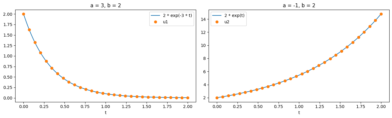
The toy model used is:

\[\frac{\mathrm{d} u}{\mathrm{d} t} = -a u\]

with initial conditions \(u(0) = b\). The model is first solved with \(a = 3, b = 2\), then with \(a = -1, b = 2\)

# Create model
model = pybamm.BaseModel()
u = pybamm.Variable("u")
a = pybamm.Parameter("a")
b = pybamm.Parameter("b")
model.rhs = {u: -a * u}
model.initial_conditions = {u: b}
model.variables = {"u": u, "a": a, "b": b}

# Set parameters, with a as an input ########################
parameter_values = pybamm.ParameterValues({"a": "[input]", "b": 2})
parameter_values.process_model(model)
#############################################################

# Discretise using default discretisation
disc = pybamm.Discretisation()
disc.process_model(model)

# Solve
t_eval = np.linspace(0, 2, 30)
ode_solver = pybamm.ScipySolver()
solution = ode_solver.solve(model, t_eval, inputs={"a": 3})

# Post-process, so that u1 can be called at any time t (using interpolation)
t_sol1 = solution.t
u1 = solution["u"]

# Solve again with different inputs ###############################
solution = ode_solver.solve(model, t_eval, inputs={"a": -1})
t_sol2 = solution.t
u2 = solution["u"]
###################################################################

# Plot
t_fine = np.linspace(0, t_eval[-1], 1000)

fig, (ax1, ax2) = plt.subplots(1, 2, figsize=(13, 4))
ax1.plot(t_fine, 2 * np.exp(-3 * t_fine), t_sol1, u1(t_sol1), "o")
ax1.set_xlabel("t")
ax1.legend(["2 * exp(-3 * t)", "u1"], loc="best")
ax1.set_title("a = 3, b = 2")

ax2.plot(t_fine, 2 * np.exp(t_fine), t_sol2, u2(t_sol2), "o")
ax2.set_xlabel("t")
ax2.legend(["2 * exp(t)", "u2"], loc="best")
ax2.set_title("a = -1, b = 2")


plt.tight_layout()
plt.show()

model.rhs

{Variable(0x5f4a102fc03b7b39, u, children=[], domains={}): Multiplication(-0x32ae6bc94fa07109, *, children=['-a', 'y[0:1]'], domains={})}

Printing parameter values

Since parameters objects must be processed by the ParameterValues class before they can be evaluated, it can be difficult to quickly check the value of a parameter that is a combination of other parameters. You can print all of the parameters (including combinations) in a model by using the print_parameters function.

a = pybamm.Parameter("a")
b = pybamm.Parameter("b")
parameter_values = pybamm.ParameterValues({"a": 4, "b": 3})
parameters = {"a": a, "b": b, "a + b": a + b, "a * b": a * b}
param_eval = parameter_values.print_parameters(parameters)
for name, value in param_eval.items():
    print(f"{name}: {value}")

a: 4.0
b: 3.0
a + b: 7.0
a * b: 12.0

If you provide an output file to print_parameters, the parameters will be printed to that output file.

References

The relevant papers for this notebook are:

pybamm.print_citations()

[1] Joel A. E. Andersson, Joris Gillis, Greg Horn, James B. Rawlings, and Moritz Diehl. CasADi – A software framework for nonlinear optimization and optimal control. Mathematical Programming Computation, 11(1):1–36, 2019. doi:10.1007/s12532-018-0139-4.
[2] Charles R. Harris, K. Jarrod Millman, Stéfan J. van der Walt, Ralf Gommers, Pauli Virtanen, David Cournapeau, Eric Wieser, Julian Taylor, Sebastian Berg, Nathaniel J. Smith, and others. Array programming with NumPy. Nature, 585(7825):357–362, 2020. doi:10.1038/s41586-020-2649-2.
[3] Scott G. Marquis, Valentin Sulzer, Robert Timms, Colin P. Please, and S. Jon Chapman. An asymptotic derivation of a single particle model with electrolyte. Journal of The Electrochemical Society, 166(15):A3693–A3706, 2019. doi:10.1149/2.0341915jes.
[4] Valentin Sulzer, Scott G. Marquis, Robert Timms, Martin Robinson, and S. Jon Chapman. Python Battery Mathematical Modelling (PyBaMM). Journal of Open Research Software, 9(1):14, 2021. doi:10.5334/jors.309.
[5] Pauli Virtanen, Ralf Gommers, Travis E. Oliphant, Matt Haberland, Tyler Reddy, David Cournapeau, Evgeni Burovski, Pearu Peterson, Warren Weckesser, Jonathan Bright, and others. SciPy 1.0: fundamental algorithms for scientific computing in Python. Nature Methods, 17(3):261–272, 2020. doi:10.1038/s41592-019-0686-2.